Experiments

With “experiment”, we refer to the systematic analysis of a RL method, the influence of its parameters onto its performance, and/or the comparison of different RL methods. Note: Even though we focus in this text onto the agent component of the world, similar experiments could also be conducted for comparing the performance of an agent in different environments.

Conducting experiments

Experiments can be either be conducted using the command line interface or using the MMLF Experimenter. For this example, download this example experiment configuration here, and extract it into your rw-directory (this should result in a directory ~/.mmlf/test_experiment). Now, you can execute the experiment using:

run_mmlf --experiment test_experiment

Note that you have to use the --experiment argument instead of --config, and the path of the experiment directory must be relative to the rw-directory. For this particular experiment, this will conduct 5 runs a 100 episodes for 3 worlds. Alternatively, you could also load the experiment into the MMLF experimenter using the “Load Experiment” button and execute it using the “Start Experiment” button. In this case, you can monitor the progress in the GUI online. See the MMLF Experimenter for more details. A further option for conducting experiments is to script them (see Scripting experiments).

The experiment configuration (in the test_experiment directory) consists of the definition of several worlds (one for each yaml-file in the worlds subdirectory of test_experiment directory) and the configuration of the experiment itself in experiment_config.yaml:

concurrency: Sequential
episodesPerRun: '100'
parallelProcesses: '1'
runsPerWorld: '5'

This configuration defines whether the experiment should be executed sequentially (“concurrency: Sequential”, i.e. only one run at a time) or concurrently (“concurrency: Concurrent”, i.e. several runs at the same time), how many episodes per world run should be conducted (“episodesPerRun”), how many runs are executed in parallel for concurrent execution order (“parallelProcesses”), and how many runs (repetitions) should be conducted for each world (“runsPerWorld”). Note that “parallelProcesses” is ignored if the execution order is sequential.

In this example experiment, three different agents are compared in the linear markov chain environment: an agent acting randomly, an TD-based agent with epsilon=0.5, and an TD-based agent with epsilon=0.1. Each of this agents acts for 100 episodes and gets 5 independent runs. By looking at the logs/linear_markov_chain directory, you may see that three novel results directories have been created (“849418770030302468” etc., see Logging for an explanation why the directories are named this way.) For convenience, you may rename these directories to more meaningful names once the experiment is finished (e.g. “Random”, “TD0.1”, and “TD0.5”). You can identify which directory belongs to which agent by looking into the world.yaml file in these directories.

Evaluating experiments

Once an experiment is finished, you can analyze it using the MMLF Experimenter. If you already conducted the experiment using the MMLF experimenter, a tab with the title “Experiment Statistics” has already been created which shows the results of the experiment. Otherwise, you can load the experiment’s results by pressing “Load Experiment Results” in the MMLF Experimenter. This opens a file selection dialog in which the root directory of the particular experiment in the RW area must be selected (logs/linear_markov_chain for the example above).

Note

It may happen that different experiments share the same root directory (namely, when both experiments use the same environment). In this case, the Experimenter cannot distinguish these experiments and interprets them as a single experiment. In order to avoid that, please copy the results of an experiment to a unique directory manually.

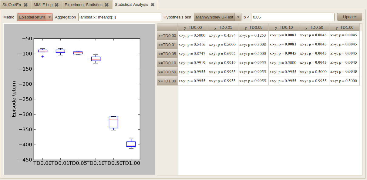
The “Experiment Statistics” tab shows you various statistics for a selected metric and allows to plot these results by pressing “Visualize”. For a more detailed explanation of the “Experiment Statistics” tab, we refer to the MMLF Experimenter. For now, the interesting part is the “Statistical Analysis” tab that is opened by pressing “Statistics” in the “Experiment Statistics” tab:

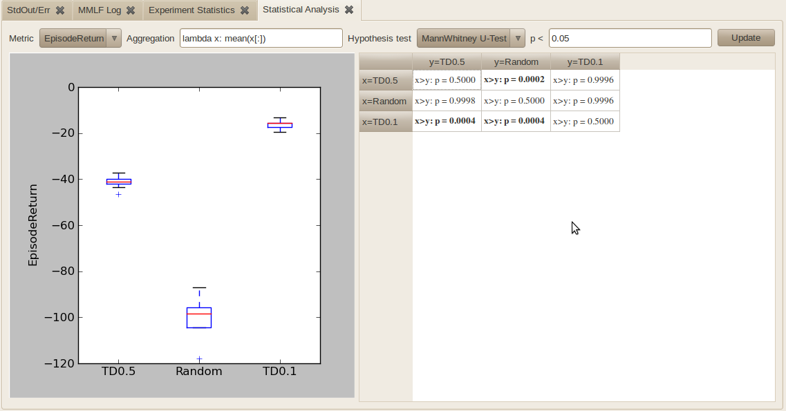
This tab shows you a boxplot based visualization of the average performance of the different setups and also a comparison based on statistical hypothesis testing. You can select the following:

• The “metric” based on which the different setups should be compared (e.g. “EpisodeReturn” or “EpisodeLength”)
• How the different values the metric takes on during a run should be combined into a single scalar value (“aggregated”). This is accomplished by using a python lambda function like “lambda x: mean(x[:])”. In this expression, the sequence of values the metric takes on during a run is stored in x (typically one value per episode). One can now select just a subset of this values using slicing (e.g. x[0:20] would just retain the first 20 values while x[:] retains all values) and choose how this value range is aggregated (mean, median, max, min are available). For instance, to compare based on the minimal performance obtained during the first 30 episodes, use “lambda x: min(x[0:30])”.
• Which statistical hypothesis test is conducted (Student t-test or MannWhitney u-test)
• Which level is considered to be significant (typically p < 0.05)

By pressing “Update”, the graphic and the significance table are updated. In the table, pairs of setups for which one setup obtained significantly better results than the other are shown bold (in the example TD0.1>TD0.5>Random)

Note

Please take care when comparing many setups: No correction for multiple testing is performed.

Scripting experiments

If a large number of agent/environments combinations should be compared it may become inconvenient to create for each combination a separate world file or to configure this world in the MMLF GUI. In such a situation it may be more convenient to write a python script that create the world configurations on the fly, execute the experiment and consolidates the log files. These python scripts use the MMLF python package interface. For example, the following script (download here) lets the TD(lambda) agent learn in the mountain car environment for six different values of the exploration ratio epsilon:

# Maja Machine Learning Framework
#
# This program is free software; you can redistribute it and/or modify
# it under the terms of the GNU General Public License as published
# by the Free Software Foundation; either version 3 of the License, or
# (at your option) any later version.

# This program is distributed in the hope that it will be useful, but
# WITHOUT ANY WARRANTY; without even the implied warranty of
# MERCHANTABILITY or FITNESS FOR A PARTICULAR PURPOSE. See the
# GNU General Public License for more details.

# You should have received a copy of the GNU General Public License
# along with this program; if not, see <http://www.gnu.org/licenses/>.

import os
import shutil
import copy
import yaml

# The mmlf must be importable (global installation or the directory into which 
# the MMLF has been extracted must be in python search path).
import mmlf
# Initialize logging and rw-area
mmlf.setupConsoleLogging()
mmlf.initializeRWArea()

# Template for world configuration
# The specific values for epsilon will be changed later, the rest remains 
# identical for all worlds
worldConfTemplateYaml = \
""" 
worldPackage : mountain_car
environment:
    moduleName : "mcar_env"
    configDict: 
        maxStepsPerEpisode : 500    
        accelerationFactor : 0.001
        maxGoalVelocity : 0.07
        positionNoise : 0.0
        velocityNoise : 0.0
agent:
    moduleName : "td_lambda_agent"
    configDict:
        gamma : 1.0
        epsilon : 0.0
        lambda : 0.95
        minTraceValue : 0.5
        stateDimensionResolution : 9
        actionDimensionResolution : 7
        function_approximator : 
            name : 'CMAC'
            number_of_tilings : 10
            learning_rate : 0.5
            update_rule : 'exaggerator'
            default : 0.0
monitor:
    policyLogFrequency : 250
"""

worldConfTemplate = yaml.load(worldConfTemplateYaml)

# Create experiment configuration
# Experiment is conducted concurrently with 8 parallel processes (if enough 
# cores are available). Each run consists of 250 episodes and 5 runs are 
# conducted per world 
experimentConf = {"concurrency": "Concurrent",
                  "episodesPerRun": '250',
                  "parallelProcesses": '8',
                  "runsPerWorld": '5',
                  "worlds" : dict()}

# Change exploration ratio of worlds
for epsilon in [0.0, 0.01, 0.05, 0.1, 0.5, 1.0]:
    worldConf = copy.deepcopy(worldConfTemplate)
    worldConf['agent']['configDict']['epsilon'] = epsilon
    experimentConf["worlds"]["TD%.2f"%epsilon] = worldConf
                        
# Run the experiment (this may take some time)
mmlf.runExperiment(experimentConf)

# Give directories more meaningful names
for worldName, worldConf in experimentConf["worlds"].items():
    # Determine log directory into which the results of a specific world 
    # have been stored. This is copy-pasted from world.py
    envConfig = worldConf['environment']
    agentConfig = worldConf['agent']
    confStr = "%s%s%s%s" % (envConfig["moduleName"],
                             sorted(zip(envConfig["configDict"].keys(),
                                        envConfig["configDict"].values())),
                             agentConfig["moduleName"],
                             sorted(zip(agentConfig["configDict"].keys(),
                                        agentConfig["configDict"].values())))
   
    directoryName = str(abs(hash(confStr)))
    
    # Rename directories
    shutil.move(os.sep.join([mmlf.getRWPath(), "logs", worldConf['worldPackage'], directoryName]),
                os.sep.join([mmlf.getRWPath(), "logs", worldConf['worldPackage'], worldName]))

You may execute this script with the following command (but be aware that this experiment may take some hours, in particular on slower machines):

python scripted_experiment.py

Instead of executing the experiment, you can also download the results that have been obtained in one execution here. Now, you may load the results into the MMLF Experimenter (using “Load Experiment Results”) and analyze them.

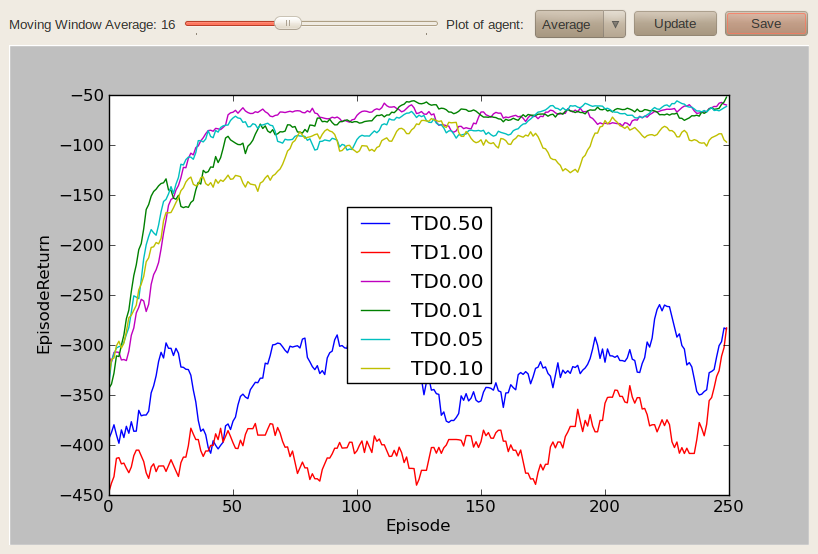
For instance, plotting the average performance of an agent after applying a moving window average of length 16:

Doing a statistical analysis of the results: